Optimization Algorithms - Code Recollection

I just completed the chapter on numerical computation in the Deep Learning book by Ian Goodfellow, Yoshua Bengio and Aaron Courville. The topic of gradient-based optimization using various algorithms is explored. The example they give at the end of the chapter is using least squares to minimize a function. This is also known as “curve-fitting”, often performed when trying to tune parameters of a model function to best match the some collected data.

Least Squares with SciPy

"Least-squares problems occur in many branches of applied mathematics. In this problem a set of linear scaling coefficients is sought that allow a model to fit data. In particular it is assumed that data $y_{i}$ is related to data $x_{i}$ through a set of coefficients $c_{j}$ and model functions $f_{j} (x_{i})$ via the model".
$y_{i} = \sum_{j} c_{j} f_{j} (x_{i}) + ϵ_{i}$ where $ϵ_{i}$ represents uncertainty in the data." [From Scipy docs]

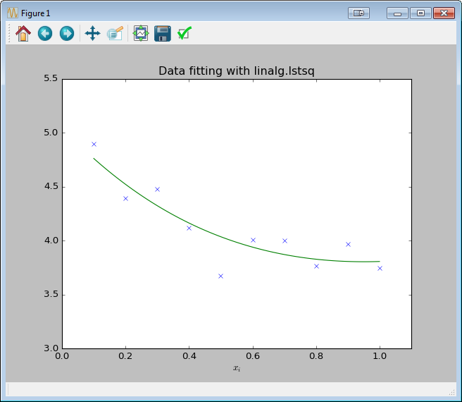
Solving directly with scipy.linalg.lstsq

import numpy as np
from scipy import linalg
import matplotlib.pyplot as plt

c1, c2 = 5.0, 2.0
i = np.r_[1:11]
xi = 0.1*i
yi = c1*np.exp(-xi) + c2*xi
zi = yi + 0.05 * np.max(yi) * np.random.randn(len(yi))

A = np.c_[np.exp(-xi)[:, np.newaxis], xi[:, np.newaxis]]
c, resid, rank, sigma = linalg.lstsq(A, zi)

xi2 = np.r_[0.1:1.0:100j]
yi2 = c[0]*np.exp(-xi2) + c[1]*xi2

plt.plot(xi,zi,'x',xi2,yi2)
plt.axis([0,1.1,3.0,5.5])
plt.xlabel('$x_i$')
plt.title('Data fitting with linalg.lstsq')
plt.show()

Solving iteratively with scipy.optimize.leastsq

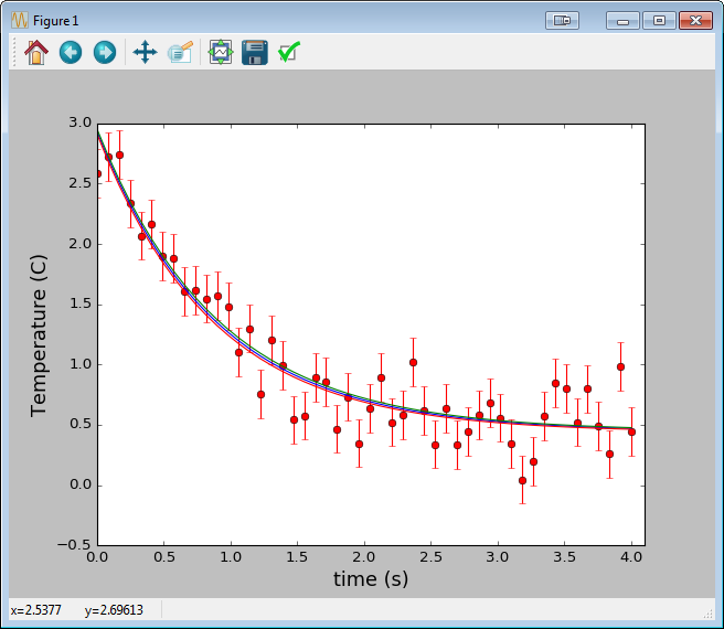
Similarly, here’s a good example of using scipy.optimize.curve_fit, a convenient wrapper around scipy.optimize.leastsq. Here we’re fitting time vs temperature data in a cooling cup of coffee.

import numpy as np
import matplotlib.pyplot as plt
from scipy.optimize import curve_fit

def fitFunc(t, a, b, c):
    return a*np.exp(-b*t) + c

t = np.linspace(0,4,50)
temp = fitFunc(t, 2.5, 1.3, 0.5)
noisy = temp + 0.25*np.random.normal(size=len(temp))

fitParams, fitCovariances = curve_fit(fitFunc, t, noisy)
print (fitParams)
print (fitCovariances)

plt.ylabel('Temperature (C)', fontsize = 16)
plt.xlabel('time (s)', fontsize = 16)
plt.xlim(0,4.1)
# plot the data as red circles with vertical errorbars
plt.errorbar(t, noisy, fmt = 'ro', yerr = 0.2)
# now plot the best fit curve and also +- 1 sigma curves
# (the square root of the diagonal covariance matrix  
# element is the uncertianty on the fit parameter.)
sigma = [fitCovariances[0,0], \
         fitCovariances[1,1], \
         fitCovariances[2,2] \
         ]
plt.plot(t, fitFunc(t, fitParams[0], fitParams[1], fitParams[2]),\
         t, fitFunc(t, fitParams[0] + sigma[0], fitParams[1] - sigma[1], fitParams[2] + sigma[2]),\
         t, fitFunc(t, fitParams[0] - sigma[0], fitParams[1] + sigma[1], fitParams[2] - sigma[2]))
plt.show()

[Code example above from the SciPy Script Repository]

← Previous Post Next Post →